Chapter 1 The Basics
All of my friends who have younger siblings who are going to college or high school - my number one piece of advice is: You should learn how to program. – Mark Zuckerberg
1.1 R and the R-Project
R is a language and an environment for statistical computing and graphics. It is a GNU project that is similar to the S language and environment, which was developed at Bell Laboratories (formerly AT&T, now Lucent Technologies) by John Chambers and his colleagues. R can be considered a different implementation of S. There are some important differences, but much code written for S runs unaltered under R.
R provides a wide variety of statistical (linear and nonlinear modeling, classical statistical tests, time-series analysis, classification, clustering, …) and graphical techniques, and is highly extensible. The S language is often the vehicle of choice for research in statistical methodology and R provides an Open Source way to participate in that activity.
1.2 R System and RStudio
RStudio is an integrated development environment (IDE) as well as a graphical user interface (GUI) for R. It includes a console, a syntax-highlighting editor that supports direct code execution as well as tools for plotting, debugging and workspace management. When you start RStudio for the first time it should look like this:
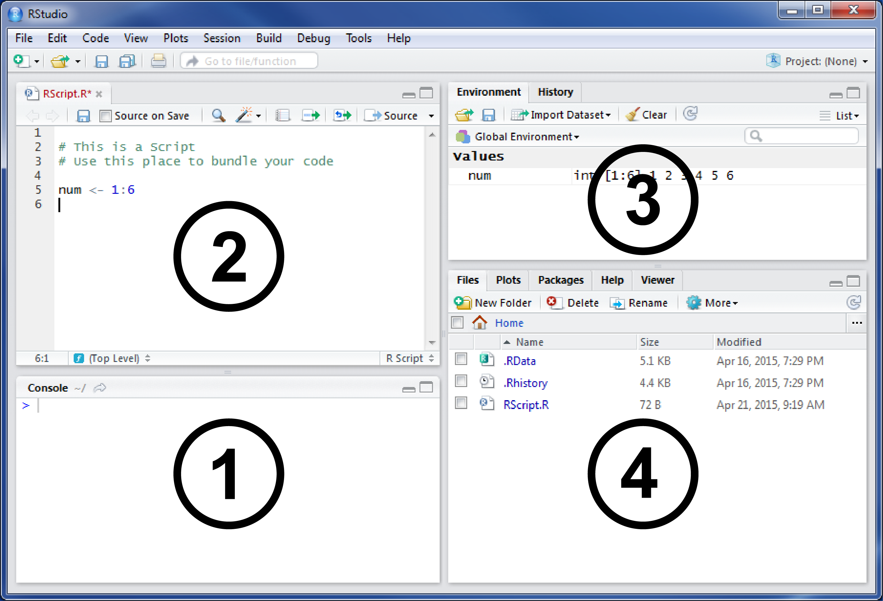
Figure 1.1: RStudio
The shown version of RStudio is 1.1.x, which was the latest one available when this script was written and revised. If you have not changed any of the default settings, your RStudio should look almost the same. The most important section is the big one on the left (1). This is the R console that connects your development environment with the R core.
RStudio makes it simple, interactive and very convenient to use R. You just type your command into the bottom line of the console tab (1), hit Enter and your computer will execute it. Commands are your way to talk to the computer and that is why the console is often also called the command line interface (CLI). The > is called the prompt and indicates that R is ready and waiting for your commands. If you type 1 + 2 into the command line, you should see the following after hitting Enter:
#R> [1] 3As we want reproducible results we need a more convenient and supporting place to work with our code. Scripts allow us to be an efficient programmer. Therefore you should bundle and work with your code in the Script Pane (2) and stop typing in the console. You can easily start a new script by clicking File \(\to\) New File \(\to\) R Script in the main menu bar. Or you hit Control + Shift + N (Windows) on the keyboard to open one automatically.
As you can see R responds to your request with more than just the result. The [1] on the left side indicates that the line in which the response is written starts with the first value. This becomes quite useful when your commands become more complex so that R returns multiple values. The colon operator (:) creates a sequence between two given numbers by incrementing the first number by 1 (or -1 respectively if the bigger number is provided as the first argument) until the second number is reached. If we want R to give back the integers between 1 and 100 we simply type1:100 and get exactly what we have asked for:
#R>   [1]   1   2   3   4   5   6   7   8   9  10  11  12  13  14  15  16  17  18
#R>  [19]  19  20  21  22  23  24  25  26  27  28  29  30  31  32  33  34  35  36
#R>  [37]  37  38  39  40  41  42  43  44  45  46  47  48  49  50  51  52  53  54
#R>  [55]  55  56  57  58  59  60  61  62  63  64  65  66  67  68  69  70  71  72
#R>  [73]  73  74  75  76  77  78  79  80  81  82  83  84  85  86  87  88  89  90
#R>  [91]  91  92  93  94  95  96  97  98  99 100
The numbers in brackets now indicate that the first line starts with the first value of R’s answer to your command and the second line starts with a higher value (depending on the size of your RStudio window). When handling matrices and bigger vectors in your programs you will greatly appreciate this small feature, but for now, we can ignore it. To make the next lines of R code more readable this formatting is only referred to when I want you to notice them. The same applies for the > at the beginning of each line. Therefore the following Code excerpts will not contain these signs, which will make it also much easier for you to copy them into your own console. To clearly differentiate between commands and responses I will indicate R’s output with R> and color them differently so that our first example will look like this:
#R> [1] 31.3 First Steps: R as Calculator
R is a powerful programming language for statistical algorithms and therefore you can also use it as a (very powerful) calculator for nearly every case you can imagine including calculations on arrays and complex matrix operations. Let us start with some basic examples:
#R> [1] 13R handles the sharp (hash) # symbol as an indicator for comments and in fact does not interpret it. You can and should (!) use it to comment on your code to express your thoughts and what you were trying to do while programming because it is necessary to understand your code. But let’s stay focused:
#R> Error: <text>:1:12: unexpected ','
#R> 1: 4 * -(5 - 1,
#R>                ^
Errors occur while programming. One of the major sources of errors is the syntax of a language. Syntax simply describes the required structure for commands. Every command has to follow certain structural rules in order to make R understand what you want it to do. In this case, R is designed to accept the point as decimal separator, otherwise, it will only prompt an error message while providing a short hint to the problem. You can then just retype the command or you can use the arrow-up key \(\uparrow\) on your keyboard to access your last command and change it accordingly:
#R> [1] -14As stated before, with R you can do everything your calculator can do, from simple mathematical operations to more complex tasks. Some well known and often used functions are:
#R> [1] 5#R> [1] 25#R> [1] 3.141593#R> [1] 0.5#R> [1] 8#R> [1] 0+8i#R> [1] 0#R> [1] 21#R> [1] 2 4 6 8 10 12#R> [1] 6Trying to calculate something that is not defined, leads to a warning. If you try dividing by zero, R reminds you that it has no answer to this question as well as any other calculator.
#R> [1] NaN1.4 Objects and Data Structures
You may have heard of objects or the concept of object-oriented programming. R is also considered to be object-oriented, which basically means that we have to deal with objects if we want to use it. You can imagine an object as a name that you can use to refer to stored data. Of course, there are rules for naming an object. Generally speaking, every symbol is possible as long as it consists of alphanumerical characters, numbers, and dots. Special characters like $, @, +, -, / or * are not allowed within names. To assign values to an object, we use the arrow <-. Whenever you tell R to handle commands containing your object, it will replace it with the data saved inside. The most basic form of an object is a variable, containing only one value:
#R> [1] 5RStudio will support you with multiple features that make your life as a programmer easier. If a new variable is generated, it will show you a sneak peek of its contents in the environment pane on the upper right corner. The environment pane (3) will show you all objects, you have created since starting RStudio.
Variable or object names are case sensitive, which means that R differentiates between small and capital letters. Two objects with the same name, but different capitalization are regarded as two different objects:
#R> [1] 6#R> [1] 4#R> [1] 2As a practical proof that different capitalization produces different objects, we can also use R to compare the created objects. You can simply do this by using == as a comparison operator. Watch out, do not forget the second equality sign. When using only one, your command will be interpreted as an assignment and has, therefore, the same effect as using <-. Although one equality sign can be used as an assignment operator, it should be avoided due to better readability of your code:
#R> [1] TRUE#R> [1] FALSE#R> [1] 1Using variables in mathematical operations does not change their values. To change stored data, you have to overwrite it. R will do this without asking for your permission. To remove a variable completely from the memory you can use the function rm().
#R> [1] 5#R> [1] 201.4.1 Data Structure: Vectors
Of course, we are not limited to storing simple numbers in R. In fact, there is no specialized data type for storing single numbers as in other programming languages. Stored single numbers are often called atomic vectors or one-element vectors. However, vectors can easily be used to store multiple numbers.
#R> [1] 1 2 3 4 5 6#R> [1] 0.5 1.0 2.0#R> [1] 0 1 2 3 4 5#R> [1] 1 4 9 16 25 36#R> [1] 2 4 6 5 7 9#R> Warning in foo + 1:5: longer object length is not a multiple of shorter object
#R> length#R> [1] 2 4 6 8 10 7As you may have noticed R does not follow the rules of matrix multiplications but uses element-wise execution instead. This means that R is applying the requested operation to each and every element of the vector. When multiplying two vectors of the same length R will always multiply the first element of the first vector with the first element of the second vector, then the second element of the first vector with the second element of the second vector and so on.
When given two vectors of different length R will repeat the shorter vector until it matches the length of the longer one. Note that the shorter vector will only be repeated within this single calculation, R does not change the vector itself. If the length of the shorter vector is not a natural multiple of the length of the long one, R will perform a calculation by concatenating the shorter vector multiple times, until it reaches the same length as the longer one, and issues a warning with the calculation results. This behavior is called vector recycling.
Element-wise operations are very useful, especially when it comes to handling data with a lot of observations. You can easily apply calculations which will only affect elements from the same observation when using vectors with the same length. If you want to know the length of a vector you can use the function length().
1.4.2 Data Structure: Matrices
Even though element-wise operations are useful sometimes you need matrix-algebra in your functions and R does of course support this, but there are special operators you have to use. There are different operators for every case you may need. You can, for example, calculate the inner product with the %*%-Operator and the outer product with the %o%-Operator.
#R> [1] 3#R> [1] 1 4 9#R> [,1]
#R> [1,] 14#R> [,1] [,2] [,3]
#R> [1,] 1 2 3
#R> [2,] 2 4 6
#R> [3,] 3 6 9When manipulating data, it may be useful to access specific columns, rows or elements of a matrix. You can simply use the row and column indices in brackets object[row, column] to access the desired data. Leaving one spot blank advises R to return all elements in this dimension. If you need to know the \(n \times m\) dimensions of the matrix you can use dim() to get to know what you need.
#R> [1] 3 3#R> [1] 1#R> [1] 2 4 6#R> [1] 3 6 9The most common way of creating matrices is using the command matrix which takes an arbitrarily long vector and input. Obviously, you need to define the number of rows and columns for the matrix. By default, all the elements from the vector are filled into the matrix column by column. To change the standard behavior we can set the argument byrow = TRUE.
#R>      [,1] [,2] [,3]
#R> [1,]    1    4    7
#R> [2,]    2    5    8
#R> [3,] 3 6 9#R> [,1] [,2] [,3]
#R> [1,] 1 2 3
#R> [2,] 4 5 6
#R> [3,] 7 8 9You can also construct matrices out of vectors manually using rbind() for row vectors and using cbind() for column vectors. Transposing a matrix can be done with t() and calculating the determinant with det():
#R>     [,1] [,2] [,3]
#R> vec    1    2    3
#R> vec    1    2    3
#R> vec 1 2 3#R> vec vec vec
#R> [1,] 1 1 1
#R> [2,] 2 2 2
#R> [3,] 3 3 3#R> [1] 0As we have already talked about comparison operators and element-wise operations it is not surprising that there are similar operations for matrices and matrix elements.
#R>     [,1] [,2] [,3]
#R> vec TRUE TRUE TRUE
#R> vec TRUE TRUE TRUE
#R> vec TRUE TRUE TRUE#R> [1] TRUEThe function all.equal() seems to be an alternative to identical() as it returns the same value for our matrix comparison. But of course, there is a reason that both of these functions exist. This has to do with the internal representation of numeric values and we are going to talk about this in more detail in the next chapter.
1.4.3 Data Structure: Strings
Data is more than just numbers and so there is a need for a structure specialized in storing sentences, words and characters, which are called strings. You can create string variables in the same way as vectors and matrices, but you need to place single or double quotation marks at the begin and end of each string.
#R> [1] "We" "love"#R> [1] "statistics"#R> [1] 1The universal length() function can also be used with string variables and it will give you the number of strings it contains and not the numbers of characters. There are many other commands for string variables e.g. dealing with putting strings together or taking them apart. The squared brackets we got to know when discussing vectors can also be used to access elements of a string.
#R> [1] 10#R> [1] 2 4#R> [1] "We" "love" "statistics"#R> [1] "statistics"1.4.4 Data Structure: Lists and Data Frames
Lists allow more complex combinations of different data types. You can see a list as a vector which can contain elements of different data types without losing information about their nature. Every sub-element in a list has an own name, like any variable or any object and can be accessed using the dollar sign $ as operator.
#R> $num
#R> [1] 1 2 3
#R>
#R> $strg
#R> [1] "abc"#R> [1] 1 2 3#R> List of 2
#R> $ num : int [1:3] 1 2 3
#R> $ strg: chr "abc"The str() command is a comfortable way of getting a quick overview of the data structure and it’s containing values of an object. It is a generic function and also works with other data structures such as simple vectors, much more complex data frames or even functions.
Data frames are a specific incarnation of lists and ideal when working with larger data sets, as they allow us to combine all sorts of data in them, which won’t work well in a normal list and won’t work at all in a matrix. Each sub-element of the data frame is handled as its own column in our matrix-like structure of data. All sub-elements need to have the same length and each sub-element needs to be consistent in terms of its data type, which results in a data frame with exactly one datatype per column and a fixed number of rows for all columns.
df <- data.frame(
  Name=c("Homer","Marge","Bart","Lisa"),
  Age=c(38 , 34 , 10 , 8),
  Sex=c("m","f","m","f"),
  stringsAsFactors = FALSE)

df                            # Display the data frame
#R> Name Age Sex
#R> 1 Homer 38 m
#R> 2 Marge 34 f
#R> 3 Bart 10 m
#R> 4 Lisa 8 f#R> [1] "Homer" "Marge" "Bart" "Lisa"1.5 Functions
1.5.1 Using Functions
Programming reveals its value when bringing data and algorithms together. We already briefly talked about the different data storing concepts, now it is time to talk about “containers” for our algorithms, which we are going to call functions. We already encountered some basic functions like sum(), sqrt() and det(), which allow us to perform basic tasks with our stored data. The base version of R includes many other and much more powerful functions, even more can be added by installing extensions, called packages, from the internet. And of course, we can write functions on our own.
A function is always defined by its name followed by a list of arguments or parameters. Most functions return a value, which can be a number, a matrix or a list. Using a function is pretty straightforward: just type in the name followed by parentheses with the data you want the function to use. Arguments can be numbers, vectors or even the output from other functions. This ability to handle the output of a function directly as an input for another function allows us to nest functions, which is also called linking.
#R> [1] 3#R> [1] 22.5#R> [1] 22Functions can handle multiple arguments as input. This allows us to specify what we want and handle different cases within the same function. But first we need to know the different arguments a function can accept - and of course, there is a function to find out about that. This function is called args(). As input, it accepts the function that you want to know the arguments of.
#R> function (x, digits = 0)
#R> NULL#R> [1] 3.14#R> Error in round(pi, length = 2): unused argument (length = 2)When using arguments not listed in the output of args(), it is quite obvious that the function can’t handle such input and produces an error. All listed arguments can be used just by assigning a value while calling the function, as it’s done above with the argument digits=2. The function works also when we do not provide a value for digits and that is why this argument is called optional. Optional arguments always have a default value like digits=0 for the function round(). Therefore, only the input to be rounded x is mandatory, so that you can not call round without providing a value for it.
The majority of functions is able to accept multiple arguments as input and there are multiple ways to pass them over, meaning you can explicitly name the arguments and assign the data to them using the =. This allows you to completely mix up the order of the arguments. Alternatively, you can pass them to the function in the right order without directly naming or addressing them. In general, it is good practice to name each argument as this keeps your code clean and understandable.
num <- c(0.5, 0.25, 0.125, 0.0625)      # Some arbitrary numbers

round(x = num, digits = 2)  # Function-call with named arguments
#R> [1] 0.50 0.25 0.12 0.06#R> [1] 0.50 0.25 0.12 0.06#R> [1] 0.50 0.25 0.12 0.06#R> [1] 2 2 2 2For some reason, people who are new to programming, feel the need to clean up the console window. As there is no real-world need for this, there is not an easy to remember command, but if you are one of those people who like it really tidy, the next example is for you:
In RStudio you can also use CTRL + L when you have placed the cursor in the console pane to clear the output area or click Clear in the global environment window.
1.5.2 Writing Functions
Programming is applied problem-solving. To start with our own function, we need a problem to solve with our newly learned R skills. And here it is:
roll() that simulates rolling a pair of dice. To implement rolling a dice you may want to use the function sample() as the heart of your program.
At first, we need the numbers located on a die. Luckily, we already know how to produce them, so this isn’t a problem at all. Next thing is to get familiar with the sample() function. We can easily do this by using args() and playing a little bit around.
#R> function (x, size, replace = FALSE, prob = NULL)
#R> NULL#R> [1] 5 3 6 4 1 2#R> [1] 1#R> [1] 5 3Using sample() only with our vector of numbers does not lead to the correct result, but the argument size allows us to adjust for the number of times a dice is rolled. We obviously need two returned values as we need one value per die, so size=2. When you run this line of code over and over again you may notice that the two returned values are never the same. If we are trying to increase the number of rolled dice, R points us directly to the reason:
#R> [1] 6 4The behavior of the sample()-function takes us directly back to one of our first statistics lessons. Every time the function returns a value it removes it from the population/sample, so it can not be returned again. If we set the option replace to TRUE the previously withdrawn number is placed back in the sample and can be drawn again. Therefore this option allows us to create independent, random samples, which is exactly what we want. We just solved our first programming problem! Now we just need to wrap our code in a function so that we can call it using roll(). For this we need the function function().
my_function <- function() { }    # This is how a function is defined

# We can simply put our working example in the function constructor,
# give it a name and execute everything by calling the given name.

roll <- function() {
  num <- 1:6
  dice <- sample(num, size = 2, replace = TRUE)
  return(dice)
}

roll()                           # We can now use our function
#R> [1] 5 3The code between the parentheses is called the body of a function. The complete code runs when you require R to execute your function. You can see how I indented these lines. This does not affect R’s behavior but makes the code a lot more readable. R ignores every blank line and space, so you can use them to structure your code.
The return() at the end of the function advises R to explicitly give back a value. Code that does not produce an output on the console by running it line by line is called a silent function. If you perform a calculation that also produces an output on the console it will be automatically returned if its the last line in your function, e.g. sum(dice) instead of return(dice) would return the combined result of the two rolled dices. Let us have a look at an overview of all the different parts of a function:
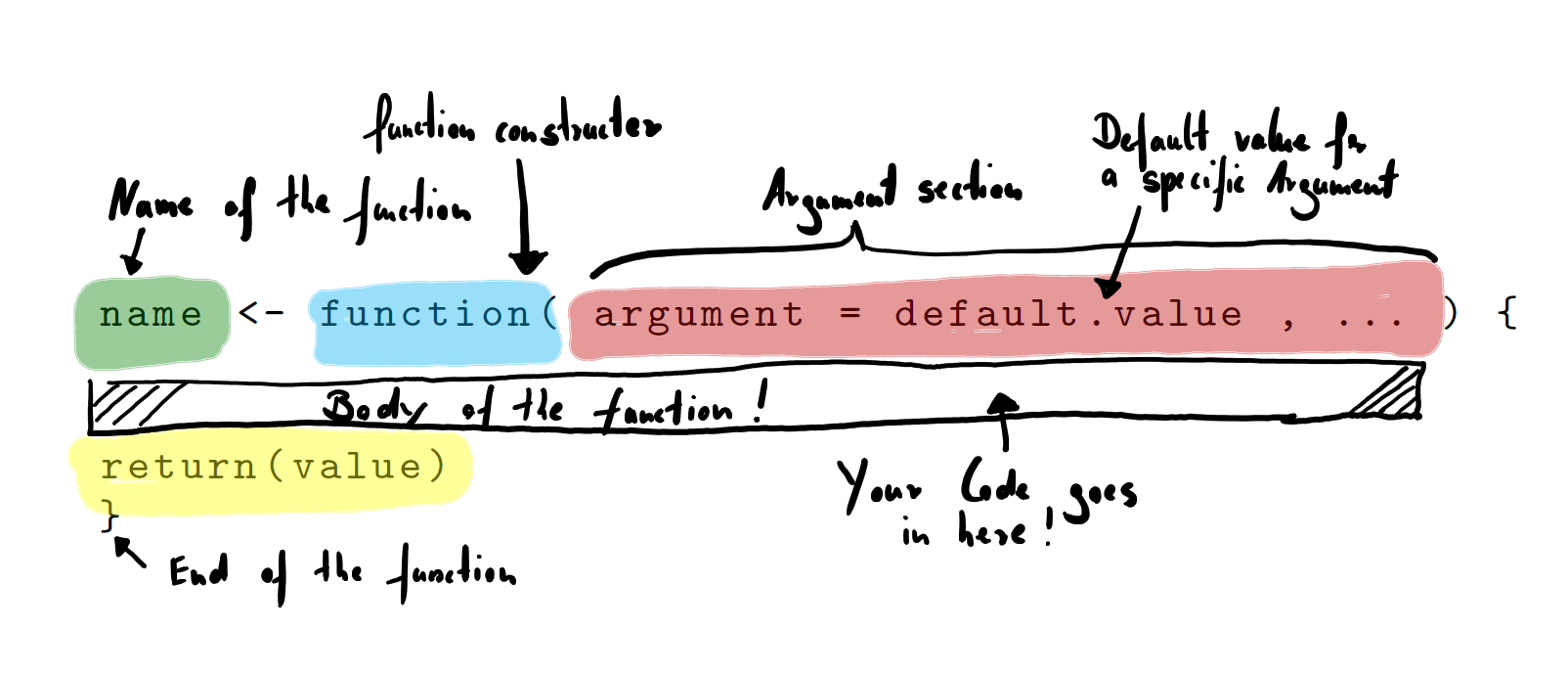
Figure 1.2: Function Constructor and Parts of a Function
1.5.3 Solving Problems
Our small roll()-function already has most of the described parts of the function constructor except for default values - in fact, it does not require any values to run the function, which makes it very inflexible. While programming, it is always better to solve general problems instead of very narrowly defined cases. So let’s adjust our problem description a little and produce a program that is more flexible.
roll() that simulates rolling a desired number of dices and allows the user to adjust the number of sides on the rolled dice.
To solve this exercise we can use our existing roll()-function and modify it to meet the desired criteria. All we have to do is define the dependencies of the sample()-function in the body arguments of the function constructor. While doing this we can also define useful default values, so that we can still use the function without arguments. Let us use rolling a six-sided pair of dice for the default values. Our improved roll()-function now looks like this:
roll <- function( num = 1:6 , rolls = 2) {
  dice <- sample(num, size = rolls, replace = TRUE)
  return(dice)
}
This function is now much more general and usable for a lot of different cases. Let’s have a brief look at how to use it. To show that the function delivers the same value when we call it with arguments and default arguments, we have to fix the random number generator. R uses this random number generator in the background to pick a value from our sample and will, therefore, deliver different results each time we call our function. Luckily we can lock the random number generator for a single execution using the set.seed() command with a freely selected numeric value as argument. Every time a routine relies on the random number generator and the seed is set to the same value R will produce the same result.
#R> [1] 1 4#R> [1] 1 4# It is easy to increase the number of rolls or the number of sides
# of the rolled dice using the argument section of the function.
roll(num = 1:18 , rolls = 5)#R> [1] 7 1 2 11 14To execute multiple lines of code at once you can simply select them and hit the Run in the upper right corner of RStudios script pane.
1.6 Packages
1.6.1 Packages with Data
Of course, we don’t need to invent everything ourselves. R comes with tons of great functions we can use for our analysis. One of the most important tasks in statistics is to perform a linear regression with one dependent and one or more independent variables.
wage1 into R and use the lm()-function to fit a linear model to the data and calculate the effect of education on wage in the simple bivariate case. Summarize and interpret your findings considering that the data was recorded back in the 1970s in the USA.
Naturally, the first step is to load the required data set into R. Luckily the data is simply available as a package that can be installed with install.packages("wooldridge"). After installation and loading the package with library(wooldridge) we can see the whole documentation including variable descriptions by typing ?wage1.
#R> [1] 526 24#R> [1] "wage" "educ" "exper" "tenure" "nonwhite" "female"
#R> [7] "married" "numdep" "smsa" "northcen" "south" "west"
#R> [13] "construc" "ndurman" "trcommpu" "trade" "services" "profserv"
#R> [19] "profocc" "clerocc" "servocc" "lwage" "expersq" "tenursq"As we can see the whole data set includes 526 observations and 24 variables. To get a first impression of the data we can type View(wooldridge::wage1). This will produce a viewer tab which can be used to view and inspect the data. Although it looks like an editable spreadsheet, the data can only be viewed and not changed. If you want to modify data you have to go back to the script view or command line and use commands to do this. If you are familiar with tools to handle spreadsheets like Excel you may think of quickly editing the data set over there and return to R afterward. If this came to your mind, just stop thinking about it now! R is much more powerful and way quicker than Excel and its lookalikes, so there is really no reason to chop up your workflow.
As we will only calculate a simple bivariate model we don’t need all the data, so we extract what we need from the big set. In our simple case, these are the columns wage containing the hourly average wages in USD of the interviewed individuals and educ their respective years of education. So we basically have to extract the first two columns from the data set.
wage      <- wooldridge::wage1$wage # Extract wage data (hourly wage in $)
education <- wooldridge::wage1$educ # Extract education data (education in years)

# Initial data inspection
summary(wage)                      # Summarize the variable wage
#R> Min. 1st Qu. Median Mean 3rd Qu. Max.
#R> 0.530 3.330 4.650 5.896 6.880 24.980#R> Min. 1st Qu. Median Mean 3rd Qu. Max.
#R> 0.00 12.00 12.00 12.56 14.00 18.00Extracting the needed columns from the data frame is easy. We already discussed the $-Operator, which allows us to address named parts of an object. After extracting the data and giving the variables comprehensive names, we should gain a condensed overview of what we are using for our analysis. The summary() command is a generic function which works for many types of data and responds with a useful summary depending on the input. In our case summary() returns typical descriptive measures. As we now have a first feeling of the data, we can construct our linear model using the lm()-function.
#R>
#R> Call:
#R> lm(formula = wage ~ 1 + education)
#R>
#R> Coefficients:
#R> (Intercept)    education
#R>     -0.9049       0.5414
When simply executing the lm()-function R only returns the parameter estimates. That is far too less to evaluate if the model is appropriate or if the estimated effects are significant. We can use the summary()-function again to gain a deeper understanding of what we have calculated and how our model looks like. For convenience and re-usability it makes sense to store the results in an own object.
model.uni <- lm(wage ~ 1 + education)  # Store results in variable
summary(model.uni)                     # Summarize the fitted model
#R>
#R> Call:
#R> lm(formula = wage ~ 1 + education)
#R>
#R> Residuals:
#R> Min 1Q Median 3Q Max
#R> -5.3396 -2.1501 -0.9674 1.1921 16.6085
#R>
#R> Coefficients:
#R> Estimate Std. Error t value Pr(>|t|)
#R> (Intercept) -0.90485 0.68497 -1.321 0.187
#R> education 0.54136 0.05325 10.167 <2e-16 ***
#R> ---
#R> Signif. codes: 0 '***' 0.001 '**' 0.01 '*' 0.05 '.' 0.1 ' ' 1
#R>
#R> Residual standard error: 3.378 on 524 degrees of freedom
#R> Multiple R-squared: 0.1648, Adjusted R-squared: 0.1632
#R> F-statistic: 103.4 on 1 and 524 DF, p-value: < 2.2e-16The summary view of the regression object model.uni gives us much more information than the lm()-function itself. This allows us to evaluate and interpret the model parameters as we have learned in our basic undergraduate statistic courses.
1.6.2 Packages with Functions
There are thousands of functions in the R core, but sometimes this is not enough and you have the need to expand R’s functionalities. As you are not the only programmer out there many of the required additional functions already exist, written by users like you, professionals or professors all around the world. And they are giving them to you for free so that you can use them for any purpose you want. So before starting a new programming project always do proper research and look at what is already out there.
Results from statistical works and analysis are often displayed using graphical tools. Producing plots of data to gain a quick aggregated overview of the data or using graphics to support your results is common, needed and useful. R is already equipped with tools to generate plots like plot() and hist() and RStudio makes them easy to use and comfortable to handle their outputs.
An additional option that aims to produce strong, nice looking plots with less effort than the standard R toolset is the package ggplot2. Their creators state that the package “takes care of many of the fiddly details that make plotting a hassle (like drawing legends)”. It seems to be worth to add ggplot2 to our portfolio. We are looking at some basics and produce some nice plots here. But first, we need to install the package. As long as you are connected to the Internet it is quite easy to install new packages using the command line:
That’s it, already. R takes care of the rest. It will visit the website, download the package and install it with all dependencies automatically and report the progress in the console. If you already know the name of a package and want to install it, you can do this by simply replacing the text in quotation marks. If you don’t know the packages name - we will discuss some resources besides your favorite search engine to find useful packages and additional help later.
Before you can use the power of a freshly installed package you have to advise R to load the package (even if it is already installed). You can do this using the library()-function. If you are trying to execute a command from the package before loading it R will respond with an error.
One of ggplot2’s most powerful functions is the ability to create quick (but nice looking) plots using qplot(). This is a generic function which produces its output dependent on its input, just like summary(). If you give qplot() a single vector it will produce a nice histogram, if you give it two vectors of equal length it will create a scatter plot.
sample <- rnorm( 1000 )         # Generate 1000 norm. dist. numbers
head(sample, 10)                # Preview the first 10 numbers
#R> [1] -1.539950042 -0.928567035 -0.294720447 -0.005767173 2.404653389
#R> [6] 0.763593461 -0.799009249 -1.147657009 -0.289461574 -0.299215118#R> Warning: `qplot()` was deprecated in ggplot2 3.4.0.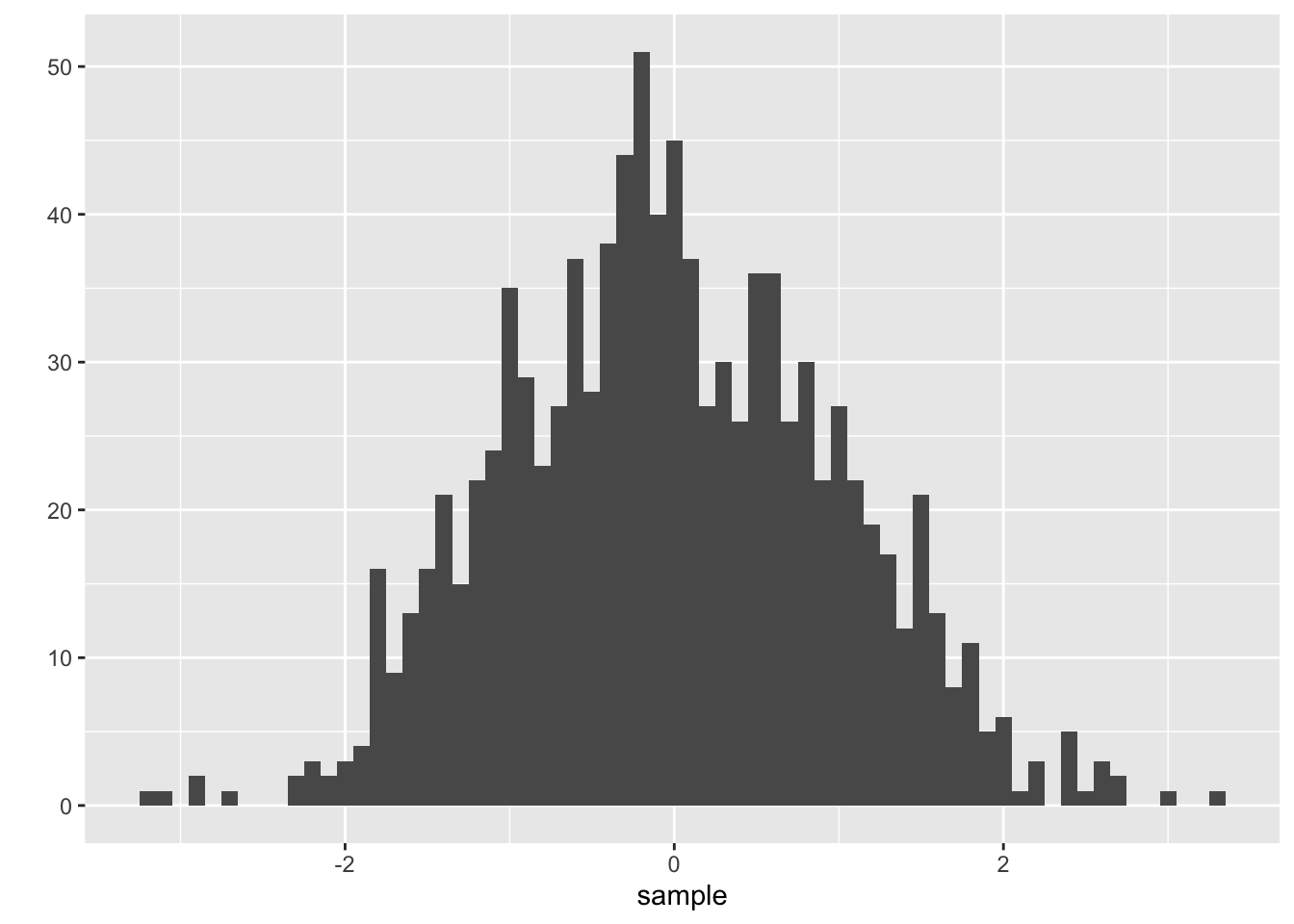
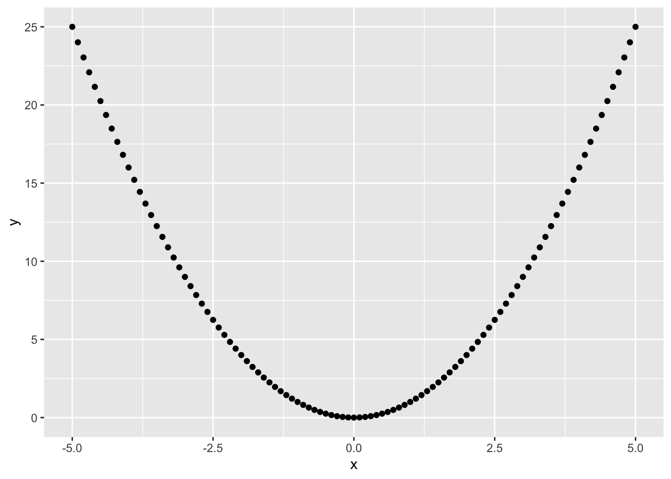
As you can see, it is very fast forward to generate nice histograms out of single vectors. The argument binwidth = .1 defines the width of each cluster to aggregate the generated values into pillars. As you may have noticed I have not written 0.1. Lazy programmers (and who isn’t?) can get rid of the leading zero and start floating point numbers with the dot. Please notice that your histogram may look a little different as rnorm() also relies on the internal random number generator and of course you can use the function hist() instead to produce a similar plot. We will dive deeper into random numbers and distributions in one of the following chapters. Let’s try out what happens if we give qplot() two vectors.
1.7 Getting Help
1.7.1 Integrated Help System
The flexible package system has a lot of advantages and puts the mind power of world-leading data scientists directly to your fingertips. When installing a new package or adding a new function which has been developed either by the R Core Team or by another developer you need to use the documentation to get used to the new functions, what they are doing in detail, how the package is used and what overlaps and problems might occur. This is exactly the reason why R has a build in help system. You can get useful information about every function you have at hand. Just place the question mark in front of the function name and hit enter or use the more formal function help().
# This is how to help yourself and find out how new or existing
# functions work. Always read the help page before asking someone!

help(sin)             # Load documentation for a function

?sin                  # Shortcut to help()

help(package=ggplot2) # Information about whole package
A help page consists of different sections, each discussing a special aspect of the function. While the exact parts of a help page vary due to different purposes of different functions the following list is not exhaustive for all functions, but you can expect to see at least the following sections:
Description: Provides a brief overview of what the function actually does or what it was intended to do. This section allows you to quickly grasp if the function is useful for your intended case.
Usage: Shows a very short function call, often just enough to see required arguments. It’s good to get easy functions to work, for more advanced applications look at the dedicated example section.
Arguments: Explains the arguments used or required by a function and gives an overview of the needed datatypes or in what way an argument manipulates the behavior of a function.
Details: Provides background information on the behavior of the function and often mentions or briefly explains the theoretical concept underlying the function.
Examples: Often the second focal point after the description section. This section provides working code examples which show in more or less detail how the function could be used in practice. Especially the combination with other functions and creation of sample data is a good source of inspiration for your own projects.
If you don’t know what the exact name of a function is you can use the help.search()-function to search for a keyword in the whole documentation. The question mark shortcut for this search function is ?? and it’s automatically suggested by R if it can’t find the function you were looking for.
1.7.2 Help on the Internet
R has a gigantic global supporter and fan base. Therefore you can find a lot about solving special problems, handling errors or information about packages by simply searching the web. Sometimes it may be difficult to search something related to R as R is at least to some people also the \(18^{th}\) letter of the alphabet and this may be confusing for your favorite search engine. Here are a few starting points which may help you on your programming journey:
- www.rseek.org
- www.stackoverflow.com
- www.r-project.org/mail.html
Exercises

EX 1
Maximiliane MustermannEX 3
Hello world!
(And all the people of the world)