Chapter 5 Transformations

Figure 5.1: Download Slides

5.1 Squared Terms in Regression Models

# First Idea
summary(mod <- lm(dist ~ 1 + speed, data = cars))

## 
## Call:
## lm(formula = dist ~ 1 + speed, data = cars)
## 
## Residuals:
##     Min      1Q  Median      3Q     Max 
## -29.069  -9.525  -2.272   9.215  43.201 
## 
## Coefficients:
##             Estimate Std. Error t value Pr(>|t|)    
## (Intercept) -17.5791     6.7584  -2.601   0.0123 *  
## speed         3.9324     0.4155   9.464 1.49e-12 ***
## ---
## Signif. codes:  0 '***' 0.001 '**' 0.01 '*' 0.05 '.' 0.1 ' ' 1
## 
## Residual standard error: 15.38 on 48 degrees of freedom
## Multiple R-squared:  0.6511, Adjusted R-squared:  0.6438 
## F-statistic: 89.57 on 1 and 48 DF,  p-value: 1.49e-12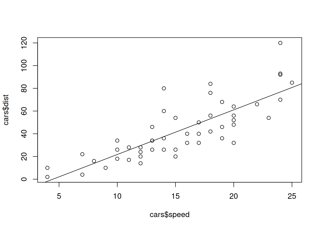

plot(cars$speed,cars$dist)
abline(mod)

# Introducing Transformations
df <- cars
df$speed_sq <- cars$speed^2

# More Models
summary(mod2 <- lm(dist ~ 1 + speed_sq, data = df))

## 
## Call:
## lm(formula = dist ~ 1 + speed_sq, data = df)
## 
## Residuals:
##     Min      1Q  Median      3Q     Max 
## -28.448  -9.211  -3.594   5.076  45.862 
## 
## Coefficients:
##             Estimate Std. Error t value Pr(>|t|)    
## (Intercept)  8.86005    4.08633   2.168   0.0351 *  
## speed_sq     0.12897    0.01319   9.781  5.2e-13 ***
## ---
## Signif. codes:  0 '***' 0.001 '**' 0.01 '*' 0.05 '.' 0.1 ' ' 1
## 
## Residual standard error: 15.05 on 48 degrees of freedom
## Multiple R-squared:  0.6659, Adjusted R-squared:  0.6589 
## F-statistic: 95.67 on 1 and 48 DF,  p-value: 5.2e-13

summary(mod3 <- lm(dist ~ 1 + speed + speed_sq, data = df))

## 
## Call:
## lm(formula = dist ~ 1 + speed + speed_sq, data = df)
## 
## Residuals:
##     Min      1Q  Median      3Q     Max 
## -28.720  -9.184  -3.188   4.628  45.152 
## 
## Coefficients:
##             Estimate Std. Error t value Pr(>|t|)
## (Intercept)  2.47014   14.81716   0.167    0.868
## speed        0.91329    2.03422   0.449    0.656
## speed_sq     0.09996    0.06597   1.515    0.136
## 
## Residual standard error: 15.18 on 47 degrees of freedom
## Multiple R-squared:  0.6673, Adjusted R-squared:  0.6532 
## F-statistic: 47.14 on 2 and 47 DF,  p-value: 5.852e-12

plot(cars$speed,cars$dist)
model <- function(x){2.47 + 0.91 * x + 0.099 * x^2}
points(1:100, sapply(1:100, model), col="red",type="l")

model_sqonly <- function(x){8.86 + 0.129 * x^2}
points(1:100, sapply(1:100,model_sqonly), col="blue",type="l")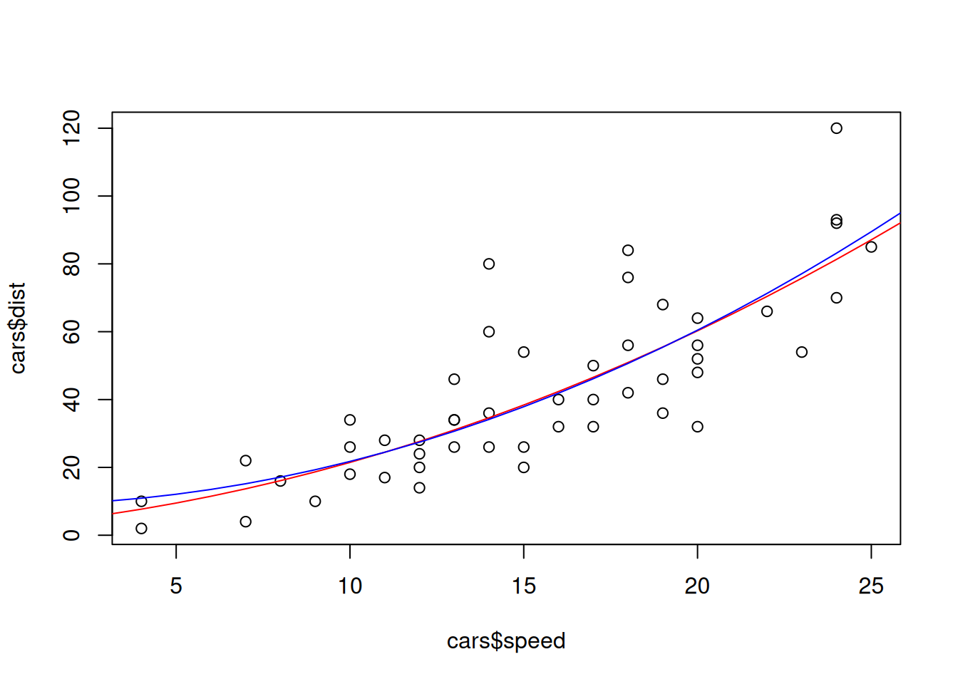

# Removing Heteroscedasticity
summary(mod4 <- lm(log(dist) ~ 1 + speed + speed_sq, data = df))

## 
## Call:
## lm(formula = log(dist) ~ 1 + speed + speed_sq, data = df)
## 
## Residuals:
##      Min       1Q   Median       3Q      Max 
## -0.97128 -0.23532 -0.02021  0.24297  0.87944 
## 
## Coefficients:
##              Estimate Std. Error t value Pr(>|t|)    
## (Intercept)  0.639838   0.406555   1.574   0.1222    
## speed        0.276815   0.055815   4.959 9.65e-06 ***
## speed_sq    -0.005167   0.001810  -2.854   0.0064 ** 
## ---
## Signif. codes:  0 '***' 0.001 '**' 0.01 '*' 0.05 '.' 0.1 ' ' 1
## 
## Residual standard error: 0.4164 on 47 degrees of freedom
## Multiple R-squared:  0.7241, Adjusted R-squared:  0.7124 
## F-statistic: 61.69 on 2 and 47 DF,  p-value: 7.177e-14

summary(mod5 <- lm(log(dist) ~ -1 + speed + speed_sq, data = df))

## 
## Call:
## lm(formula = log(dist) ~ -1 + speed + speed_sq, data = df)
## 
## Residuals:
##      Min       1Q   Median       3Q      Max 
## -0.76424 -0.26184  0.00965  0.30250  0.98119 
## 
## Coefficients:
##            Estimate Std. Error t value Pr(>|t|)    
## speed     0.3611914  0.0157595  22.919  < 2e-16 ***
## speed_sq -0.0077104  0.0008271  -9.322  2.4e-12 ***
## ---
## Signif. codes:  0 '***' 0.001 '**' 0.01 '*' 0.05 '.' 0.1 ' ' 1
## 
## Residual standard error: 0.4228 on 48 degrees of freedom
## Multiple R-squared:  0.9869, Adjusted R-squared:  0.9863 
## F-statistic:  1808 on 2 and 48 DF,  p-value: < 2.2e-16

summary(mod5 <- lm(log(dist) ~ -1  + speed_sq, data = df))

## 
## Call:
## lm(formula = log(dist) ~ -1 + speed_sq, data = df)
## 
## Residuals:
##     Min      1Q  Median      3Q     Max 
## -2.2594 -0.1085  0.8586  1.6941  2.5656 
## 
## Coefficients:
##           Estimate Std. Error t value Pr(>|t|)    
## speed_sq 0.0107233  0.0006599   16.25   <2e-16 ***
## ---
## Signif. codes:  0 '***' 0.001 '**' 0.01 '*' 0.05 '.' 0.1 ' ' 1
## 
## Residual standard error: 1.446 on 49 degrees of freedom
## Multiple R-squared:  0.8435, Adjusted R-squared:  0.8403 
## F-statistic: 264.1 on 1 and 49 DF,  p-value: < 2.2e-16

# TODO: Add final plot

5.2 Elasticity

An elasticity coefficient is the ratio of the percentage change in the forecast variable (\(y\)) to the percentage change in the predictor variable (\(x\)). Mathematically, the elasticity is defined as \((dy/dx)\times(x/y)\). Consider the log-log model, \[ \log y=\beta_0+\beta_1 \log x + \varepsilon. \] Express \(y\) as a function of \(x\) and show that the coefficient \(\beta_1\) is the elasticity coefficient.

\[ \log(y) = \beta_0 + \beta_1 \log(x) + \varepsilon \qquad \mid \mathbb{E}(\cdot \mid x)\] Taking the conditional expectation on the left and right hand side of the quation

\[\mathbb{E}(\log(y) \mid x) = \mathbb{E}(\beta_0 + \beta_1 \log(x) + \varepsilon \mid x)\] leads to the following as \(\mathbb{E}(\varepsilon\mid x) = 0\).

\[ \log(y) = \beta_0 + \beta_1 \log(x) \qquad \mid \frac{\partial}{\partial x}\] After taking derivatives of the left and right side with respect to \(x\) we receive. The left hand side follows due to the implicit differentiation.

\[ \frac{\partial}{\partial x}\log(y) = \frac{\partial}{\partial x}(\beta_0 + \beta_1 \log(x))\]

\[\frac{\partial\log(y)}{\partial x} = 0 + \beta_1 \frac{1}{x}\] \[\frac{1}{y} \frac{\partial y}{\partial x} = \beta_1 \frac{1}{x} \qquad \mid \cdot x\]

After rearranging we get the definition of the the elasticity.

\[\beta_1 = \frac{x}{y} \frac{\partial y}{\partial x}\]